The Simple Math Behind Image Rotation

I recently started learning videogame development and stumbled upon the topic of sprite animation. As I was goofing around with pixel-based (raster) image rotations, I wondered how the earliest game developers tackled this problem.

Thankfully, we have a time machine (the internet) that lets us travel back and find out exactly that. One thing led to another, and I gathered enough information and made plenty of sketches to explore the mathematics behind image rotation in this essay.

If you are the type who is curious about the technical side of animation or are just someone who enjoys math, this essay is right up your alley. I will keep it beginner-friendly; I promise! Why don’t we start by figuring out what the title image is all about?

The Pixel Salad

Most digital images that we see today, be it on our phones, televisions, or monitors, are pixel-based images (formally known as raster graphics). They approximate objects and scenes that make sense to our brains using a rectangular grid, whose dimensions we refer to as resolution.

We call each rectangular geometrical element in this grid a pixel, and each pixel carries exactly one colour value (a combination of red, green, and blue). When you and I see typical high resolution digital images today, our eyes cannot perceive the individual pixels and our brains are tricked into thinking that we are actually seeing the objects represented by those pixels.

For instance, as you are reading this essay, your brain probably thinks that you are reading printed words of some sort, but in reality, what you are reading are pixels that approximate how printed words would look like.

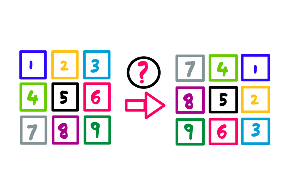
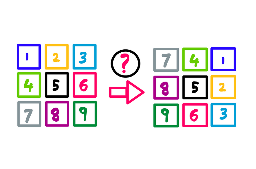
All this is cool. But what does this have to with the title image? A lot! You see, the title image represents a simplified image that has only 9 pixels in a 3×3 square grid. Imagine you zoomed into a high-resolution image until you landed on a 3×3 pixel-grid like this.

For convenience, I have numbered each pixel. Now, depending upon the device you are using to read this essay, you might have needed to scroll back up to see the title image again. You wouldn’t believe this, but technology has progressed so much that it allows me to reproduce the title image once more below for your convenience.

Notice the pixel-grid on the right. Focus on the colours and numbers, and you will realise that the pixel-grid (our simplified image, essentially) is rotated 90° in the clockwise direction (I haven’t rotated the numbers for ease of reading).

We are now about to explore the mathematics that makes this possible. Imagine that we are videogame developers back in the late 80’s. The algorithm that I am about to show you was very popular back then.

But getting into the nitty-gritty math can be hard for some folks. So, I will start by explaining the algorithm using an intuitive approach. When the water gets warm enough, we will get into the math.

The Old School Raster Rotation Algorithm

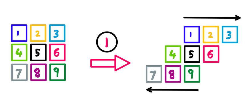
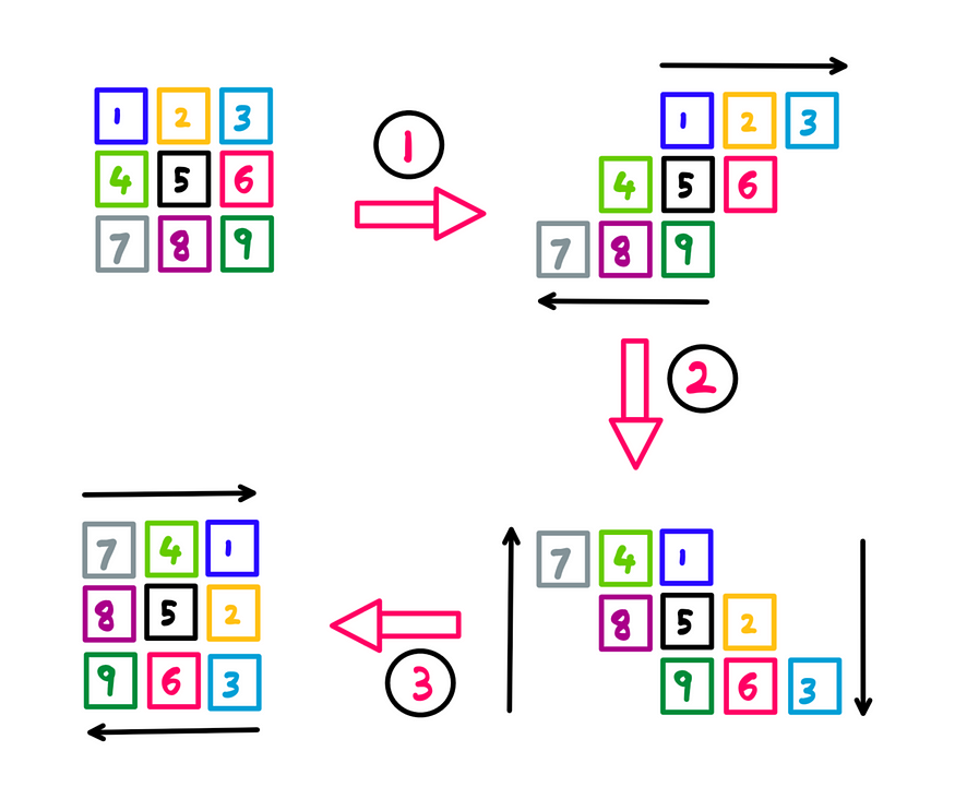
This algorithm works in three steps. Take a look at the first step here:

What we are doing here is as follows:

1. Move the top row (with pixels 1, 2, and 3) to the right by one pixel-width.
2. Move the bottom row (with pixels 7, 8, and 9) to the left by one pixel-width.
3. The center-row remains as is.

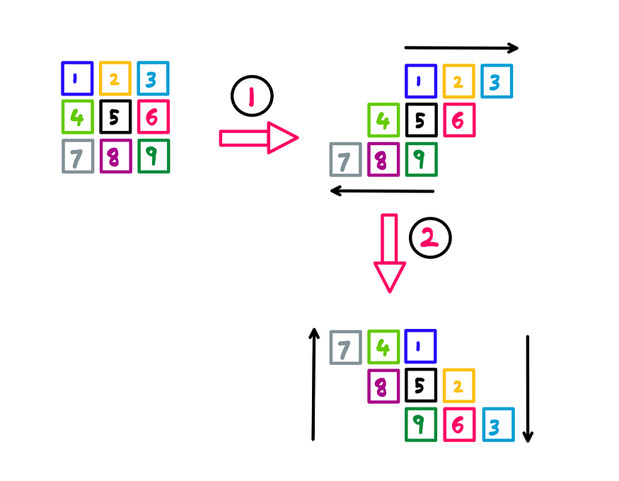
Now, onto the second step:

We are dealing with columns here as opposed to rows in step 1. The summary is as follows:

1. Move the left-most column (with pixel 7) up by two column-heights.

2. Move the second-left column (with pixels 4 and 8) up by one column-height.

3. The central column (with pixels 1, 5, and 9) remains as is.

4. Move the second-right column (with pixels 2 and 6) down by one column-height.

5. Move the right-most column (with pixel 3) down by two column-heights.

Finally, we arrive at step 3:

Step 3 is easy; we essentially go through the same procedure as in step 1, but apply them to the results of step 2. For completion, here is the summary:

1. Move the top row (with pixels 7, 4, and 1) to the right by one pixel-width.

2. Move the bottom row (with pixels 9, 6, and 3) to the left by one pixel-width.

3. The center-row remains as is.

And voila! We have now rotated the original (3×3 pixel-grid) image clockwise by 90°. We are off to a great start in terms of intuition, but we still need to explore the math behind these steps. Let us do just that.

---

The Math behind the Old School Raster Image Rotation

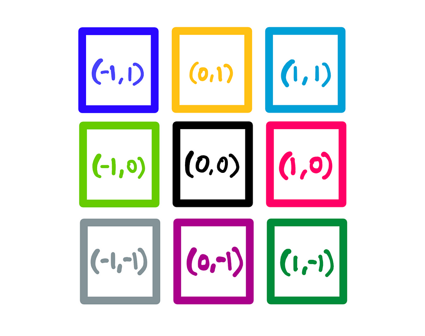
To start exploring the math, I am making one small change to the starting pixel-grid. Instead of numbering each pixel, I am assigning (x, y) cartesian coordinates to each pixel.

The center (black) pixel becomes the origin, with x-coordinate = 0, and y-coordinate = 0. All pixels to its right take positive x-coordinates, and all pixels above it take positive y-coordinates. Negative-coordinates are symmetrical and each pixel is 1 unit wide and 1 unit high.

This essay is supported by Generatebg

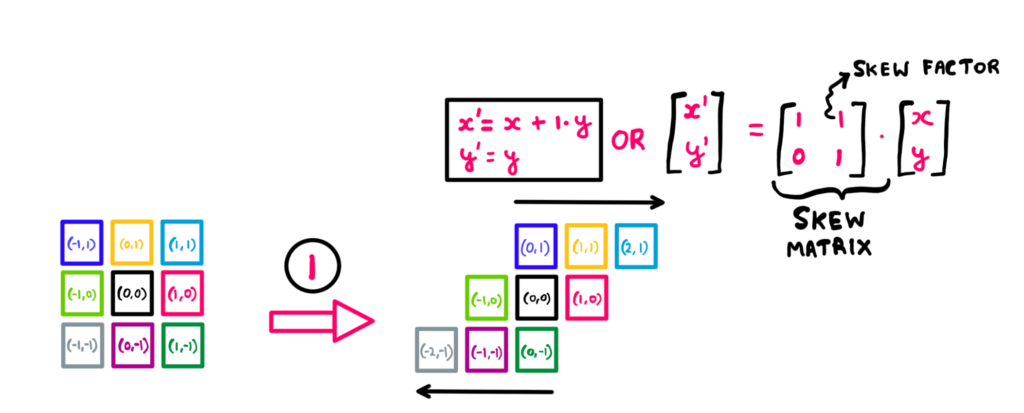
Now that we have established a more conducive mathematical model, let us take a look at the math behind step 1:

The summary here is as follows:

1. We recalculate a new x-coordinate for each pixel using the expression x’ = x + (1 * y).

2. We keep the y-coordinate for all pixels as is.

Since we don’t alter y-coordinates, we are moving pixels only in the horizontal direction.

As all pixels in the the top row have y-coordinate = 1, they get pushed to the positive x-direction by 1 pixel width (we multiply y with 1 pixel width).

Similarly, as all pixels in the bottom row have y-coordinate = -1, they get pushed to the negative x-direction by 1 pixel width.

In formal terms, we are skewing the pixel-grid. In physics/mechanics terms, we are shearing the raster image in the x-direction. We can achieve the same effect by considering x- and y-coordinates as a vector and multiplying it by a skew/shear matrix as you see in the image.

Since we are pushing the pixels by 1 pixel-width, the shear/skew factor here is 1. That is it for step 1.

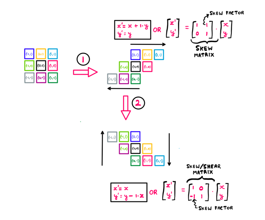
You might have already imagined how step 2 would pan out. Here it is:

The summary for step 2 is as follows:

1. We keep the x-coordinate for all pixels as is.

2. We recalculate a new y-coordinate for each pixel using the expression y’ = y – (1 * x).

Since, we don’t change any x-coordinate, all the skewing/shearing happens in the vertical direction this time around. Also, notice that we are shearing in the negative direction (as opposed to the positive-direction with step 1).

There is no deep meaning here; this is how this algorithm works. We need to reverse the direction in step 2, or we will not get the desired rotation.

Similar to step 1, we could easily come up with a simplified skew/shear matrix (which has a skew factor of -1 due to the direction change).

Finally, we move on to the easiest step of them all — step 3:

I bet you’ve figured out step 3 by now. It is essentially the same as step 1, but applied to the result of step 2. We are simply shearing the result of step 2 in the horizontal direction to get the final desired rotation.

And voila! There we have the math behind raster image rotation.

But at the beginning of this essay, I did mention that videogame developers used this algorithm in the late 80’s and 90’s. What do folks use nowadays to rotate raster images?

The Rotation Matrix

These days, we achieve image rotation by simply multiplying each pixel’s coordinates using a matrix known as the rotation matrix:

To be formal, this is a specific rotation matrix that belongs to a whole family of rotation matrices that make use of the properties of Sine and Cosine. This particular one rotates vectors in the clockwise direction by 90° (a tensor operation, if you will).

When we follow this “algorithm”, we do the entire rotation neatly in a single step. Yet, why did videogame developers back in the 80’s and 90’s not use this approach?

It is not that they were dumb to not have figured it out back then; rotation matrices are much older. The real reason has to do with computational capacity back in the 80’s and 90’s.

Computers back then were not nearly as powerful as the ones we have today (computer hardware has been improving exponentially over time thus far). As a consequence, employing the rotation matrix was computationally intensive, as computing Sines and Cosines involved floating point operations.

As opposed to this, the old raster rotation algorithm (originally developed by Alan Paeth) was a “hack” that involved simple arithmetic calculations and took advantage of the fact that matrix multiplication is not commutative. As a result, game developers could gain performance by employing this algorithm with ‘int’-type numbers.

In fact, this algorithm is so efficient that many image editing tools use it even today!

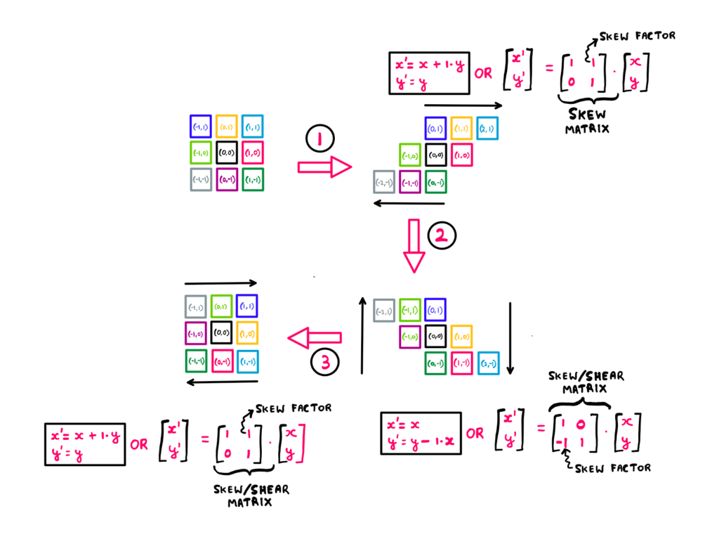
For those who are wondering how shear/skew is related to rotation (since we skewed the picture thrice to achieve rotation), here are steps 1 through 3 using horizontal and vertical shear matrices:

Note that we are shearing by 45° here to achieve a net rotation of 90°.

I hope you enjoyed our little exploration into the math behind raster image rotation!

---

If you’d like to get notified when interesting content gets published here, consider subscribing.

Further reading that might interest you: 

• How To Resolve The Three Threes Problem?
• Why Do We Really Use Euler’s Number For Growth?
• How To Actually Subtract Using Addition?

If you would like to support me as an author, consider contributing on Patreon.

---

Reference: Alan Paeth